Note
Go to the end to download the full example code.
Gradients of Excitability and Recurrence Revealed by Stimulation Mapping and Whole-Brain Modelling#
This example gives a replication and didactic explanation of the multi-site Steroetactic (s)EEG modelling and results reported in Momi et al. (Nature Comms 2025).
The code includes data fetching, model fitting, and result visualization based on the methods presented in the paper.
Please read our paper, and if you use this code, please cite it:
Momi D.,…,…. Griffiths J.D. (2025). “Gradients of Excitability in Human Cortex Revealed by Stimulation Mapping and Whole-Brain Modelling.” eLife, doi: 10.7554/eLife.83232.
0. Overview of study and summary of key results#
The human brain exhibits a modular and hierarchical structure, spanning low-order sensorimotor to high-order cognitive/affective systems. What is the mechanistic significance of this organization for brain dynamics and information processing properties? We investigated this question using rare simultaneous multimodal electrophysiology (stereotactic and scalp electroencephalography - EEG) recordings in 36 patients with drug-resistant focal epilepsy during presurgical intracerebral electrical stimulation (iES) (323 stimulation sessions). Our analyses revealed an anatomical gradient of excitability across the cortex, with stronger iES-evoked EEG responses in high-order compared to low-order regions. Mathematical modelling further showed that this variation in excitability levels results from a differential dependence on recurrent feedback from non-stimulated regions across the anatomical hierarchy, and could be extinguished by suppressing those connections in-silico. High-order brain regions/networks thus show an activity pattern characterized by more inter-network functional integration than low-order ones, which manifests as a spatial gradient of excitability that is emergent from, and causally dependent on, the underlying hierarchical network structure. These findings offer new insights into how hierarchical brain organization influences cognitive functions and could inform strategies for targeted neuromodulation therapies.
Study Overview#

A. Intracerebral electrical stimulation (iES) applied to an intracortical target region generates an early (~20-30 ms) response (evoked-related potential (ERP) waveform component) at high-density scalp electroencephalography (hd-EEG) channels sensitive to that region and its immediate neighbors (red arrows). This also appears in more distal connected regions after a short delay due to axonal conduction and polysynaptic transmission. Subsequent second (~60–80 ms) and third (~140–200 ms) late evoked components are frequently observed (blue arrows). After identifying the stimulated network in this way, we aim to determine the extent to which this second component relies on intrinsic network activity versus recurrent whole-brain feedback.
B. Schematic of the hierarchical spatial layout of canonical RSNs as demonstrated in Margulies and colleagues12, spanning low-order networks showing greater functional segregation to high-order networks showing greater functional integration15. Networks are distributed based on their position along the first principal gradient. The stimulation sites are distributed across different levels of this gradient.
C. Schematic of virtual dissection methodology and key hypotheses tested. We first fit personalized connectome-based computational models of iES-evoked responses to the hd-EEG time series, for each patient and stimulation location. Then, precisely timed communication interruptions (virtual dissections) were introduced to the fitted models, and the resulting changes in the iES-evoked propagation pattern were evaluated. We hypothesized that lesioning would lead to activity suppression (C, right side) in high-order but not low-order networks.
Results#

A. The histogram illustrates the distance in centimeters between the electrode’s centroid delivering the electrical stimulus and the center of the nearest Schaefer’s parcel. The results indicate a high level of spatial precision, with 97.2% of sessions showing distances of less than 1 cm.
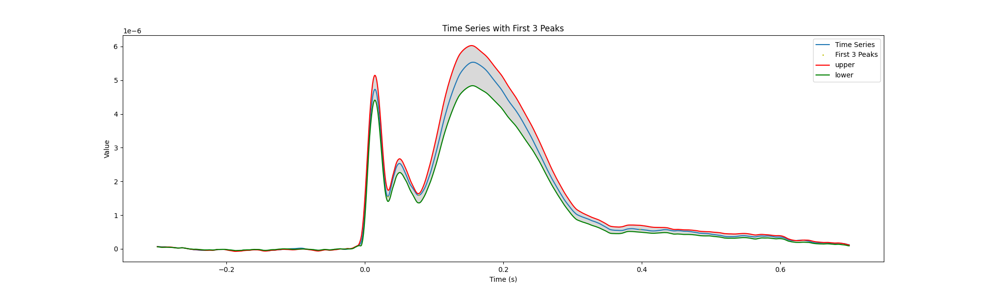
B. Global mean field power (GMFP) of hd-EEG averaged across all 36 subjects and 323 sessions, revealing three consistent response peaks/clusters within strict confidence intervals at ~40 ms, ~80 ms, and ~370 ms, consistent with prior electrophysiological research.
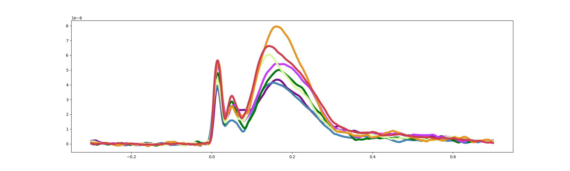
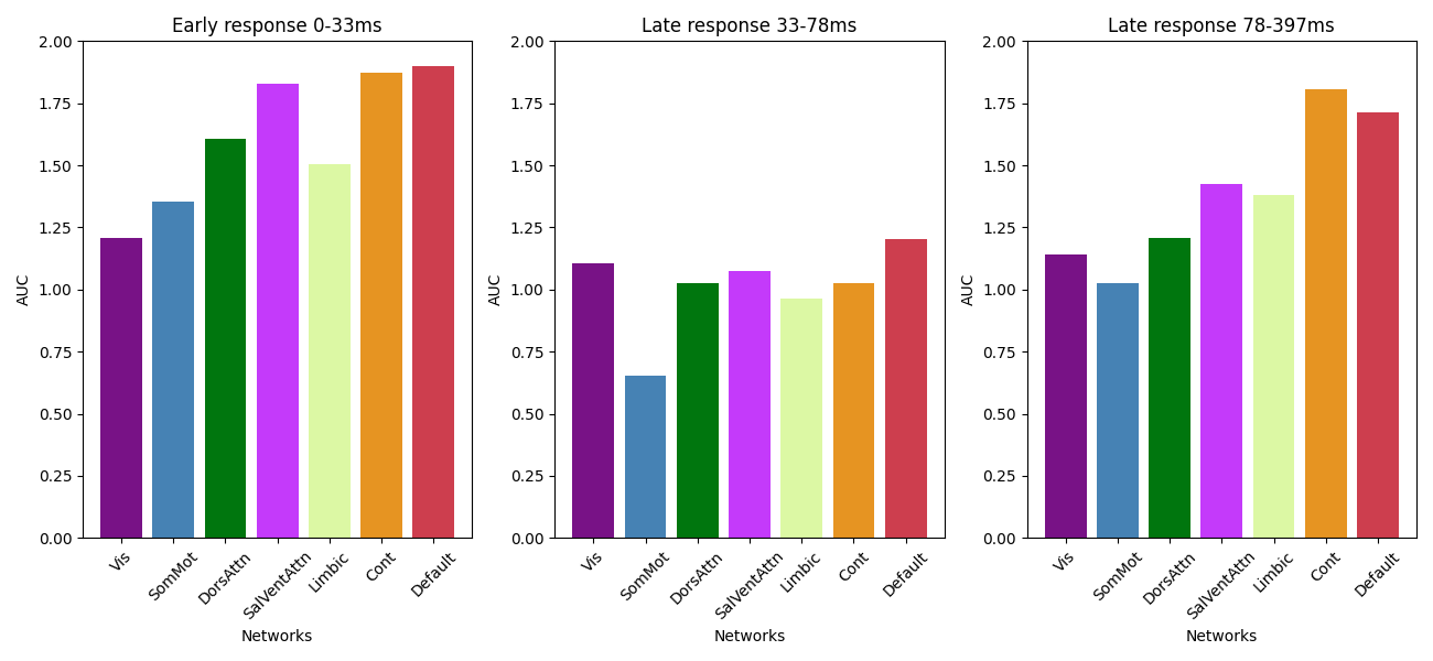
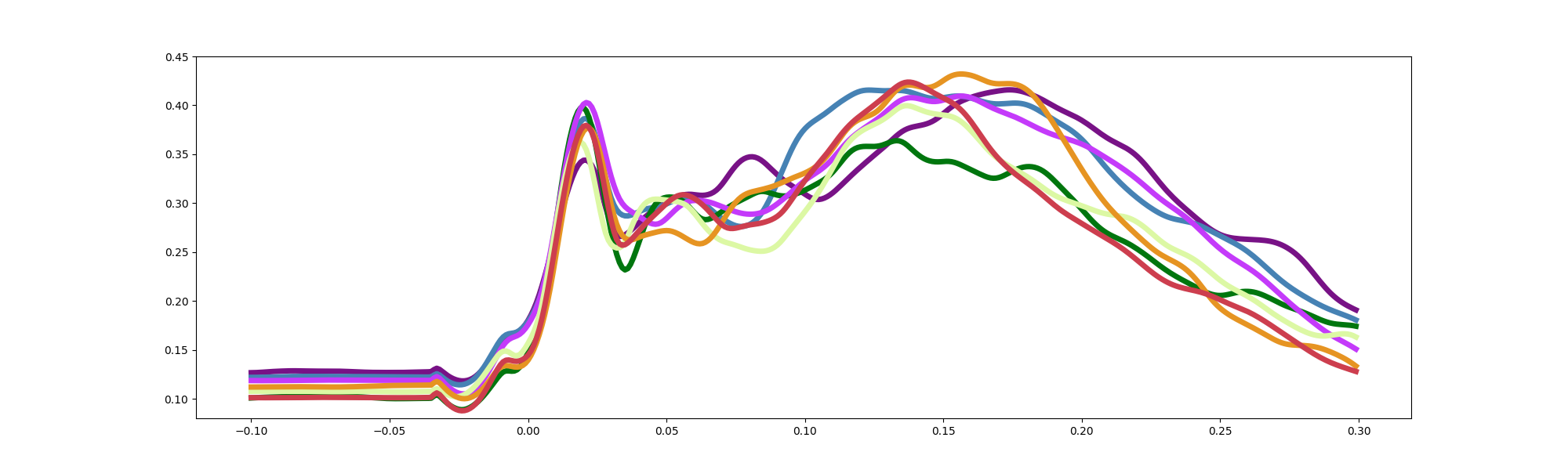
C. GMFP of every stimulated Resting-State Network (RSN) for hd-EEG (top row) and sEEG (bottom row). The bar plot of the normalized area under the curve (AUC) of the three clusters revealed a significantly stronger global activation pattern when the stimulus targeted high-order networks, such as the Default mode network (DMN) and Frontoparietal Network (FPN), particularly for the late evoked responses (third cluster at ~370 ms). Data are presented as mean values ± standard error of the mean (SEM) (error bars), with individual subject data points overlaid (36 independent subjects, 323 stimulation sessions). In the GMFP time course plots, shaded areas represent ±SEM around the mean. Notably, this trend aligns with the “principal gradient” hierarchy reported in the functional magnetic resonance imaging (fMRI) literature, which describes a general pattern from low-order to high-order regions

A. Global mean field power (GMFP) for every stimulated network for model-generated high-density electroencephalography (hd-EEG) data run with both the intact (continuous line) and disconnected (dashed line) structural connectome. Findings show a more pronounced decrease in evoked late responses for high-order networks (LN: Limbic Network, SN: Salience Network, DAN: Dorsal attention network, FPN: Frontoparietal Network, DMN: Default mode network).
B. Area under the curve (AUC) differences comparing the simulation run with the intact versus the lesioned structural connectome. The bar plot shows differences across three time windows (1st response: 0−37 ms, 2nd response: 37–78 ms, 3rd response: 78–373 ms). Data are presented as mean values ± standard error of the mean (SEM) (error bars), with individual subject data points overlaid (36 independent subjects, 323 stimulation sessions). A significant reduction in the AUC was found for late responses (78−373 ms) of high-order networks (LN, SN, DAN, FPN, and DMN) compared to low-order networks (Visual Network [VN] and Somatomotor Network [SMN]), indicated by asterisks (*P < 0.05).
C. Demonstration of the network recurrence-based theory for two representative sessions. Simulations of evoked dynamics are run using the intact (left) and lesioned (right) anatomical connectome. In the latter case, the connections were removed to isolate the stimulated networks for SMN (top) and DMN (bottom). In the case of the low-order network, this virtual dissection does not significantly impact the evoked potentials, while for the high-order network, a substantial reduction or disappearance of evoked components was observed.
Conclusions#
Using a computational framework recently developed for personalized neurostimulation modelling.
Using model to uncover neural states across netoworks: able to study how the brain signals propagate across networks
Using model as a simulator to mimic patient dynamics and potential treatment effects.
1. Setup#
Importage
# General imports
import os
import sys
import json
import time
import warnings
warnings.filterwarnings('ignore')
import re
import math
import glob
import pickle
import requests

# Python imports
import numpy as np
import pandas as pd
import scipy
import scipy.io
from scipy.signal import find_peaks
import sklearn

# Plot imports
import matplotlib.pyplot as plt
import seaborn as sns

# Imaging imports
import mne
import nibabel
import nibabel as nib
from nilearn import plotting, surface
from nilearn.image import load_img

# WHOBPYT imports
import torch
import whobpyt
from whobpyt.datasets.fetchers import fetch_egmomi2025
from whobpyt.depr.momi2025.jansen_rit import par, Recording, method_arg_type_check, dataloader
from whobpyt.depr.momi2025.jansen_rit import RNNJANSEN, ParamsJR, CostsJR, Model_fitting
Download data
data_folder = fetch_egmomi2025()
2 - Model fitting and key results#
2.1 Empirical Data Analysis#
Loading data
start_time = time.time() # For estimating run time of the empirical analysis
# Loading network colour filw from the GitHub URL
url = 'https://github.com/Davi1990/DissNet/raw/main/examples/network_colour.xlsx'
colour = pd.read_excel(url, header=None)[4]
# Evoked data
all_eeg_evoked = np.load(data_folder + '/empirical_data/all_eeg_evoked.npy')
# Epoched example
epo_eeg = mne.read_epochs(data_folder + '/empirical_data/example_epoched.fif', verbose=False)
# GFMA data
all_gfma = np.zeros((all_eeg_evoked.shape[0], all_eeg_evoked.shape[2]))

for ses in range(all_eeg_evoked.shape[0]):
    all_gfma[ses,:] =  np.std(all_eeg_evoked[ses,:,:],axis=0) #np.mean(np.mean(epo_eeg._data, axis=0),axis=0)
    # Normalized to the baseline for comparison
    all_gfma[ses,:] = np.abs(all_gfma[ses,:] - np.mean(all_gfma[ses, :300]))

# Load Schaefer 1000 parcels 7 networks
with open(data_folder + '/empirical_data/dist_Schaefer_1000parcels_7net.pkl', 'rb') as handle:
    dist_Schaefer_1000parcels_7net = pickle.load(handle)
# Extract the stimulation region data from the loaded pickle file
stim_region = dist_Schaefer_1000parcels_7net['stim_region']
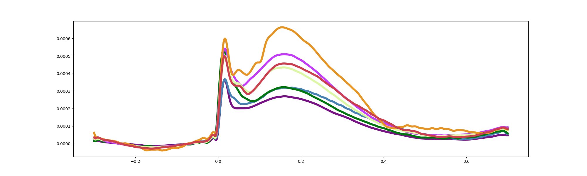
Plot evoked EEG GFMA at each network
# 7 networks definition
networks = ['Vis', 'SomMot', 'DorsAttn', 'SalVentAttn', 'Limbic', 'Cont', 'Default']
# Create a dictionary to store the network indices
stim_network_indices = {network: [] for network in networks}
# Iterate over stim region
for i, label in enumerate(stim_region):
    # Iterate over each network
    for network in networks:
        if network in label:
            stim_network_indices[network].append(i)
            break

net_gfma = {}
# Iterate over each network
for network in networks:
    # GFMA for each network
    net_gfma[network] = all_gfma[stim_network_indices[network]]

# Get the GFMA averages for each network
averages = []
for key, value in net_gfma.items():
    average = sum(value) / len(value)
    averages.append(average)

averages = np.array(averages)


# Define the desired figure size
fig = plt.figure(figsize=(20, 6))

# Plot the data
for net in range(len(networks)):
    plt.plot(epo_eeg.times, averages[net, :] - np.mean(averages[net, :300]), colour[net], linewidth=5)

# Display the plot
plt.show()
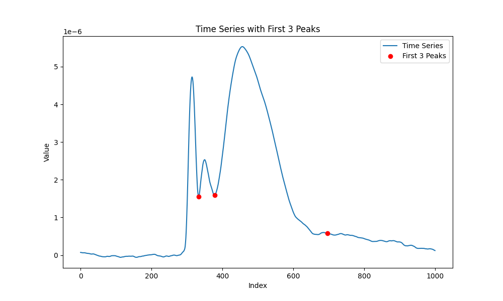
Plot peaks
# Calculate the mean array
time_series = np.mean((averages[:, :] - np.mean(averages[:, :300])), axis=0)

# Find peaks in the time series data
peaks, _ = find_peaks(-time_series[:700], distance=1)  # Adjust 'distance' parameter as needed

peak_values = time_series[peaks]

# Get the indices of the first 3 peaks in descending order of amplitude
first_3_peak_indices = peaks[np.argsort(peak_values)[::-1][:3]]

# Get the actual values of the first 3 peaks
first_3_peak_amplitudes = peak_values[np.argsort(peak_values)[::-1][:3]]

# Plot the time series and the identified peaks
plt.figure(figsize=(10, 6))
plt.plot(time_series, label='Time Series')
plt.plot(first_3_peak_indices, first_3_peak_amplitudes, 'ro', label='First 3 Peaks')
plt.legend()
plt.xlabel('Index')
plt.ylabel('Value')
plt.title('Time Series with First 3 Peaks')
plt.show()
Plot evoked response variation across sessions
# Assuming you have a 2D array all_gfma with shape (323, 1001)
# Calculate the mean and standard deviation along the first axis (sessions)
mean_all_gfma = np.mean(all_gfma, axis=0)
std_all_gfma = np.std(all_gfma, axis=0)
# Calculate the margin of error for the confidence interval
confidence_level = 0.95
z_score = 1.96  # For a 95% confidence interval
margin_of_error = z_score * (std_all_gfma / np.sqrt(len(all_gfma)))

# Calculate the upper and lower bounds of the confidence interval
upper_bound = mean_all_gfma + margin_of_error
lower_bound = mean_all_gfma - margin_of_error

upper_bound =upper_bound - np.mean(upper_bound[:300])
lower_bound =lower_bound - np.mean(lower_bound[:300])

if len(epo_eeg.times) == len(time_series):
    # Plot the time series and the identified peaks
    plt.figure(figsize=(20, 6))
    plt.plot(epo_eeg.times, time_series, label='Time Series')
    plt.plot(epo_eeg.times[first_3_peak_indices], first_3_peak_amplitudes, 'yo', markersize=1, label='First 3 Peaks')
    plt.plot(epo_eeg.times, upper_bound,'-r', label='upper')
    plt.plot(epo_eeg.times, lower_bound,'-g', label='lower')
    plt.fill_between(epo_eeg.times, upper_bound, lower_bound, color="k", alpha=0.15)  # Use 'epo_eeg.times'
    plt.legend()
    plt.xlabel('Time (s)')  # Set the x-axis label to 'Time (s)'
    plt.ylabel('Value')
    plt.title('Time Series with First 3 Peaks')
    #plt.savefig('C:/Users/davide_momi/Desktop/peaks.png', dpi=300)
    plt.show()
else:
    print("The lengths of 'epo_eeg.times' and 'time_series' don't match.")
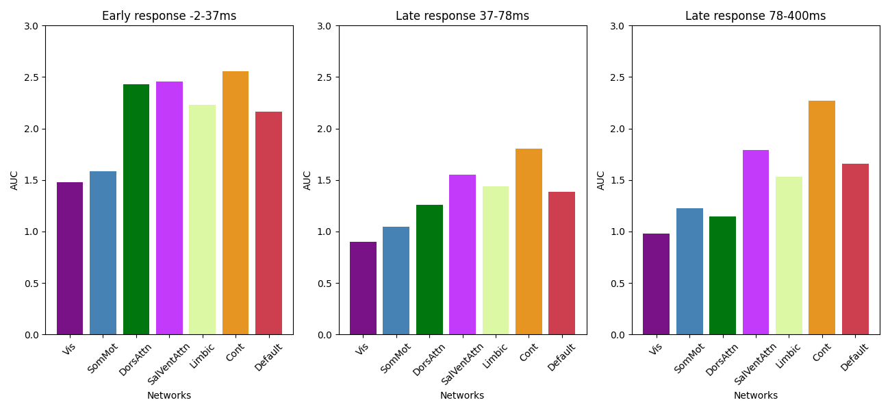
Plot AUC
windows = 3
AUC = np.zeros((3,all_gfma.shape[0]))

first_3_peak_indices_sorted = sorted(first_3_peak_indices)
first_peak = epo_eeg.times[first_3_peak_indices_sorted[0]]
second_peak = epo_eeg.times[first_3_peak_indices_sorted[1]]
third_peak = epo_eeg.times[first_3_peak_indices_sorted[2]]

for ses in range(all_gfma.shape[0]):
    AUC[0, ses] = np.trapz(all_gfma[ses, np.where(epo_eeg.times==0)[0][0]:np.where(epo_eeg.times==first_peak)[0][0]]
                           - np.mean(all_gfma[ses, :300]), dx=5)
    AUC[1, ses] = np.trapz(all_gfma[ses, np.where(epo_eeg.times==first_peak)[0][0]:np.where(epo_eeg.times==second_peak)[0][0]]
                           - np.mean(all_gfma[ses, :300]), dx=5)
    AUC[2, ses] = np.trapz(all_gfma[ses, np.where(epo_eeg.times==second_peak)[0][0]:np.where(epo_eeg.times==third_peak)[0][0]]
                           - np.mean(all_gfma[ses, :300]), dx=5)

AUC[0,:] = AUC[0,:] / (first_3_peak_indices_sorted[0] - 300)
AUC[1,:] = AUC[1,:] / (first_3_peak_indices_sorted[1] - first_3_peak_indices_sorted[0])
AUC[2,:] = AUC[2,:] / (first_3_peak_indices_sorted[2] - first_3_peak_indices_sorted[1])


net_AUC = {}

# Iterate over each network
for network in networks:
    # AUC for each network
    net_AUC[network] = AUC[:,stim_network_indices[network]]

# Obtain the average AUC
AUC_averages = np.zeros((len(networks), windows))
for idx, key in enumerate(net_AUC.keys()):
    AUC_averages[idx, :] = np.mean(net_AUC[key], axis=1)

AUC_averages = AUC_averages *100000


# Create the figure and subplots
fig, axs = plt.subplots(1, 3, figsize=(13, 6))  # 2 rows, 1 column

# Plot in the first subplot
axs[0].bar(range(AUC_averages[:, 1].shape[0]), AUC_averages[:, 0], color=colour)
axs[0].set_xticks(range(AUC_averages[:, 0].shape[0]))
axs[0].set_xticklabels(networks, rotation=45)
axs[0].set_xlabel('Networks')
axs[0].set_title('Early response 0-' + str(round(first_peak*1000)) + 'ms')
axs[0].set_ylabel('AUC')
axs[0].set_ylim(0, 2)  # Adjust the y-axis limits as needed

# Plot in the second subplot (same as the first subplot)
axs[1].bar(range(AUC_averages[:, 1].shape[0]), AUC_averages[:, 1], color=colour)
axs[1].set_xticks(range(AUC_averages[:, 0].shape[0]))
axs[1].set_xticklabels(networks, rotation=45)
axs[1].set_xlabel('Networks')
axs[1].set_title('Late response ' + str(round(first_peak*1000)) + '-' + str(round(second_peak*1000)) + 'ms')
axs[1].set_ylabel('AUC')
axs[1].set_ylim(0, 2)  # Adjust the y-axis limits as needed

# Plot in the second subplot (same as the first subplot)
axs[2].bar(range(AUC_averages[:, 2].shape[0]), AUC_averages[:, 2], color=colour)
axs[2].set_xticks(range(AUC_averages[:, 0].shape[0]))
axs[2].set_xticklabels(networks, rotation=45)
axs[2].set_xlabel('Networks')
axs[2].set_title('Late response ' + str(round(second_peak*1000)) + '-' + str(round(third_peak*1000)) + 'ms')
axs[2].set_ylabel('AUC')
axs[2].set_ylim(0, 2)  # Adjust the y-axis limits as needed

plt.tight_layout()  # Adjust the spacing between subplots if needed

plt.show()
Plot sEEG at each network
# Load sEEG epochs
with open(data_folder + '/empirical_data/all_epo_seeg.pkl', 'rb') as handle:
    all_epo_seeg = pickle.load(handle)

all_gfma = np.zeros((len(list(all_epo_seeg.keys())), epo_eeg._data.shape[2]))

for ses in range(len(list(all_epo_seeg.keys()))):
    epo_seeg =all_epo_seeg[list(all_epo_seeg.keys())[ses]]
    for xx in range(epo_seeg.shape[0]):
        epo_seeg[xx,:] = epo_seeg[xx,:] - np.mean(epo_seeg[xx,:300])

    all_gfma[ses,:] =  np.std(epo_seeg, axis=0)

# Load Schaefer 1000 parcels
with open(data_folder + '/empirical_data/dist_Schaefer_1000parcels_7net.pkl', 'rb') as handle:
    dist_Schaefer_1000parcels_7net = pickle.load(handle)
# Extract the stimulation region data from the loaded pickle file
stim_region = dist_Schaefer_1000parcels_7net['stim_region']

networks = ['Vis', 'SomMot', 'DorsAttn', 'SalVentAttn', 'Limbic', 'Cont', 'Default']
# Create a dictionary to store the network indices
stim_network_indices = {network: [] for network in networks}
for i, label in enumerate(stim_region):
    # if dist_Schaefer_1000parcels_7net['dist'][i] < 7:
            # Iterate over each network
            for network in networks:
                if network in label:
                    stim_network_indices[network].append(i)
                    break


net_gfma = {}
# Iterate over each network
for network in networks:
    # GFMS for each network
    net_gfma[network] = all_gfma[stim_network_indices[network]]

# Compute the GFMA averages
averages = []
for key, value in net_gfma.items():
    average = sum(value) / len(value)
    averages.append(average)

averages = np.array(averages)

# Download the network colour file from the GitHub URL
url = 'https://github.com/Davi1990/DissNet/raw/main/examples/network_colour.xlsx'
colour = pd.read_excel(url, header=None)[4]

# Define the desired figure size
fig = plt.figure(figsize=(20, 6))

# Plot the data
for net in range(len(networks)):
    plt.plot(epo_eeg.times, averages[net, :] - np.mean(averages[net, :300]), colour[net], linewidth=5)

# Display the plot
plt.show()
Plot sEEG AUC
# Calculate the mean array as you mentioned
time_series = np.mean((averages[:, :] - np.mean(averages[:, :300])), axis=0)

# Find peaks in the time series data
peaks, _ = find_peaks(-time_series, width=15)  # Adjust 'distance' parameter as needed

peak_values = time_series[peaks]

# Get the indices of the first 3 peaks in descending order of amplitude
first_3_peak_indices = peaks[np.argsort(peak_values)[::-1][:3]]
first_3_peak_indices = np.array([298, 337, 378, 700])
first_3_peak_amplitudes = time_series[first_3_peak_indices]

windows = 3
AUC = np.zeros((3,all_gfma.shape[0]))

first_peak = epo_eeg.times[first_3_peak_indices[0]]
second_peak = epo_eeg.times[first_3_peak_indices[1]]
third_peak = epo_eeg.times[first_3_peak_indices[2]]
fourth_peak = epo_eeg.times[first_3_peak_indices[3]]

for ses in range(all_gfma.shape[0]):
    AUC[0, ses] = np.trapz(all_gfma[ses, np.where(epo_eeg.times==first_peak)[0][0]:np.where(epo_eeg.times==second_peak)[0][0]]
                           - np.mean(all_gfma[ses, :300]), dx=5)
    AUC[1, ses] = np.trapz(all_gfma[ses, np.where(epo_eeg.times==second_peak)[0][0]:np.where(epo_eeg.times==third_peak)[0][0]]
                           - np.mean(all_gfma[ses, :300]), dx=5)
    AUC[2, ses] = np.trapz(all_gfma[ses, np.where(epo_eeg.times==third_peak)[0][0]:np.where(epo_eeg.times==fourth_peak)[0][0]]
                           - np.mean(all_gfma[ses, :300]), dx=5)


AUC[0,:] = AUC[0,:] / 33
AUC[1,:] = AUC[1,:] / 45
AUC[2,:] = AUC[2,:] / 319

net_AUC = {}
# Iterate over each network
for network in networks:
    # AUC for each network
    net_AUC[network] = AUC[:,stim_network_indices[network]]

# Obtain AUC averages
AUC_averages = np.zeros((len(networks), windows))
for idx, key in enumerate(net_AUC.keys()):
    AUC_averages[idx, :] = np.mean(net_AUC[key], axis=1)

AUC_averages = AUC_averages*1000
# AUC_averages = (AUC_averages / np.max(AUC_averages, axis=0)) * 100


# Create the figure and subplots
fig, axs = plt.subplots(1, 3, figsize=(13, 6))  # 2 rows, 1 column

# Plot in the first subplot
axs[0].bar(range(AUC_averages[:, 1].shape[0]), AUC_averages[:, 0], color=colour)
axs[0].set_xticks(range(AUC_averages[:, 0].shape[0]))
axs[0].set_xticklabels(networks, rotation=45)
axs[0].set_xlabel('Networks')
axs[0].set_title('Early response '+ str(round(first_peak*1000)) + '-' + str(round(second_peak*1000)) + 'ms')
axs[0].set_ylabel('AUC')
axs[0].set_ylim(0, 3)  # Adjust the y-axis limits as needed

# Plot in the second subplot (same as the first subplot)
axs[1].bar(range(AUC_averages[:, 1].shape[0]), AUC_averages[:, 1], color=colour)
axs[1].set_xticks(range(AUC_averages[:, 0].shape[0]))
axs[1].set_xticklabels(networks, rotation=45)
axs[1].set_xlabel('Networks')
axs[1].set_title('Late response ' + str(round(second_peak*1000)) + '-' + str(round(third_peak*1000)) + 'ms')
axs[1].set_ylabel('AUC')
axs[1].set_ylim(0, 3)  # Adjust the y-axis limits as needed

# Plot in the third subplot (same as the first subplot)
axs[2].bar(range(AUC_averages[:, 2].shape[0]), AUC_averages[:, 2], color=colour)
axs[2].set_xticks(range(AUC_averages[:, 0].shape[0]))
axs[2].set_xticklabels(networks, rotation=45)
axs[2].set_xlabel('Networks')
axs[2].set_title('Late response ' + str(round(third_peak*1000)) + '-' + str(round(fourth_peak*1000)) + 'ms')
axs[2].set_ylabel('AUC')
axs[2].set_ylim(0, 3)  # Adjust the y-axis limits as needed

plt.tight_layout()
plt.show()

end_time = time.time()
elapsed_time = end_time - start_time
print(f"Elapsed time: {elapsed_time} seconds")
Elapsed time: 5.20625376701355 seconds
2.2 Model fitting#
# Select the session number to use: Please do not change it as we are using subject-specific anatomy
ses2use = 10

# Load the precomputed EEG evoked response data from a file
all_eeg_evoked = np.load(data_folder + '/empirical_data/all_eeg_evoked.npy')

# Read the epoch data from an MNE-formatted file
epo_eeg = mne.read_epochs(data_folder + '/empirical_data/example_epoched.fif', verbose=False)

# Compute the average evoked response from the epochs
evoked = epo_eeg.average()

# Replace the data of the averaged evoked response with data from the selected session
evoked.data = all_eeg_evoked[ses2use]

# Load additional data from pickle files
with open(data_folder + '/empirical_data/all_epo_seeg.pkl', 'rb') as handle:
    all_epo_seeg = pickle.load(handle)

with open(data_folder + '/empirical_data/dist_Schaefer_1000parcels_7net.pkl', 'rb') as handle:
    dist_Schaefer_1000parcels_7net = pickle.load(handle)

# Extract the stimulation region data from the loaded pickle file
stim_region = dist_Schaefer_1000parcels_7net['stim_region']

# Load Schaefer 200-parcel atlas data from a URL
url = 'https://raw.githubusercontent.com/ThomasYeoLab/CBIG/master/stable_projects/brain_parcellation/Schaefer2018_LocalGlobal/Parcellations/MNI/Centroid_coordinates/Schaefer2018_200Parcels_7Networks_order_FSLMNI152_2mm.Centroid_RAS.csv'
atlas = pd.read_csv(url)

# Extract coordinates and ROI labels from the atlas data
coords_200 = np.array([atlas['R'], atlas['A'], atlas['S']]).T
label = atlas['ROI Name']

# Remove network names from the ROI labels for clarity
label_stripped_200 = []

for xx in range(len(label)):
    label_stripped_200.append(label[xx].replace('7Networks_', ''))

# Load Schaefer 1000-parcel atlas data from a URL
url = 'https://raw.githubusercontent.com/ThomasYeoLab/CBIG/master/stable_projects/brain_parcellation/Schaefer2018_LocalGlobal/Parcellations/MNI/Centroid_coordinates/Schaefer2018_1000Parcels_7Networks_order_FSLMNI152_2mm.Centroid_RAS.csv'
atlas = pd.read_csv(url)

# Extract coordinates and ROI labels from the atlas data
coords_1000 = np.array([atlas['R'], atlas['A'], atlas['S']]).T
ROI_Name = atlas['ROI Name']

# Remove network names from the ROI labels for clarity
label_stripped_1000 = []

for xx in range(len(ROI_Name)):
    label_stripped_1000.append(ROI_Name[xx].replace('7Networks_', ''))

# Find the index of the stimulation region in the list of stripped ROI labels (1000 parcels)
stim_idx = label_stripped_1000.index(stim_region[ses2use])

# Use the index to get the coordinates of the stimulation region from the 1000-parcel atlas
stim_coords = coords_1000[stim_idx]

# Extract the network name from the stimulation region label
# The network name is the part after the underscore in the stimulation region label
stim_net = stim_region[ses2use].split('_')[1]


# Define distance function
def euclidean_distance(coord1, coord2):
    x1, y1, z1 = coord1[0], coord1[1], coord1[2]
    x2, y2, z2 = coord2[0], coord2[1], coord2[2]
    return math.sqrt((x2 - x1)**2 + (y2 - y1)**2 + (z2 - z1)**2)

# Initialize an empty list to store distances
distances = []

# Iterate over each coordinate in the 200-parcel atlas
for xx in range(coords_200.shape[0]):
    # Compute the Euclidean distance between the current coordinate and the stimulation coordinates
    # Append the computed distance to the distances list
    distances.append(euclidean_distance(coords_200[xx], stim_coords))

# Convert the list of distances to a NumPy array for easier manipulation
distances = np.array(distances)

# Iterate over the indices of the distances array, sorted in ascending order
for idx, item in enumerate(np.argsort(distances)):
    # Check if the network name of the stimulation region is present in the label of the current parcel
    if stim_net in label_stripped_200[item]:
        # If the condition is met, assign the index of the current parcel to `parcel2inject`
        parcel2inject = item
        # Exit the loop since the desired parcel has been found
        break

# Extract the absolute values of the EEG data for the specified session
abs_value = np.abs(all_epo_seeg[list(all_epo_seeg.keys())[ses2use]])

# Normalize each time series by subtracting its mean
for xx in range(abs_value.shape[0]):
    abs_value[xx, :] = abs_value[xx, :] - np.mean(abs_value[xx, :])

# Take the absolute value of the normalized data
abs_value = np.abs(abs_value)

# Find the starting and ending points around the maximum value in the data
# Get the index of the maximum value along the time axis
starting_point = np.where(abs_value == abs_value.max())[1][0] - 10
ending_point = np.where(abs_value == abs_value.max())[1][0] + 10

# Compute the maximum, mean, and standard deviation of the data within the range around the maximum
max_value = np.max(abs_value[:, starting_point:ending_point])
mean = np.mean(abs_value[:, starting_point:ending_point])
std = np.std(abs_value[:, starting_point:ending_point])

# Define a threshold as mean + 4 times the standard deviation
thr = mean + (4 * std)

# Count the number of unique regions affected by the threshold
number_of_region_affected = np.unique(np.where(abs_value > thr)[0]).shape[0]

# Load the rewritten Schaeffer 200 parcels
img = nib.load(data_folder + '/calculate_distance/example_Schaefer2018_200Parcels_7Networks_rewritten.nii')

# Get the shape and affine matrix of the image
shape, affine = img.shape[:3], img.affine

# Create a meshgrid of voxel coordinates
coords = np.array(np.meshgrid(*(range(i) for i in shape), indexing='ij'))

# Rearrange the coordinates array to have the correct shape
coords = np.rollaxis(coords, 0, len(shape) + 1)

# Apply the affine transformation to get the coordinates in millimeters
mm_coords = nib.affines.apply_affine(affine, coords)

# Initialize an array to store the coordinates of the 200 parcels
sub_coords = np.zeros((3, 200))

# Loop over each parcel (1 to 200)
for xx in range(1, 201):
    # Find the voxel coordinates where the parcel value equals the current parcel number
    vox_x, vox_y, vox_z = np.where(img.get_fdata() == xx)

    # Calculate the mean coordinates in millimeters for the current parcel
    sub_coords[:, xx - 1] = np.mean(mm_coords[vox_x, vox_y, vox_z], axis=0)


# Initialize an empty list to store distances
distances = []

# Compute the Euclidean distance between each coordinate in the 200-parcel atlas and the coordinate of the parcel to inject
for xx in range(coords_200.shape[0]):
    distances.append(euclidean_distance(sub_coords[:,xx], sub_coords[:,parcel2inject]))

# Convert the list of distances to a NumPy array for further processing
distances = np.array(distances)

# Find the indices of the closest parcels to inject, based on the number of affected regions
inject_stimulus = np.argsort(distances)[:number_of_region_affected]

# Compute stimulus weights based on the distances
# Adjust distances to a scale of 0 to 1 and calculate the values for the stimulus weights
values = (np.max(distances[inject_stimulus] / 10) + 0.5) - (distances[inject_stimulus] / 10)

# Initialize an array for stimulus weights with zeros
stim_weights_thr = np.zeros((len(label)))

# Assign the computed values to the stimulus weights for the selected parcels
stim_weights_thr[inject_stimulus] = values

old_path = data_folder + "/anatomical/example-bem"
new_path = data_folder + "/anatomical/example-bem.fif" # CS

if not os.path.exists(new_path):
    os.rename(old_path, new_path)
    print(f"Renamed {old_path} to {new_path}")

# File paths for transformation, source space, and BEM files
trans = data_folder + '/anatomical/example-trans.fif'
src = data_folder + '/anatomical/example-src.fif'
#bem = 'anatomical/example-bem'
bem = data_folder + '/anatomical/example-bem.fif'

# Create a forward solution using the provided transformation, source space, and BEM files
# Only EEG is used here; MEG is disabled
fwd = mne.make_forward_solution(epo_eeg.info, trans=trans, src=src, bem=bem,
                                meg=False, eeg=True, mindist=5.0, n_jobs=2,
                                verbose=False)

# Extract the leadfield matrix from the forward solution
leadfield = fwd['sol']['data']

# Convert the forward solution to a fixed orientation with surface orientation
fwd_fixed = mne.convert_forward_solution(fwd, surf_ori=True, force_fixed=True,
                                         use_cps=True)
# Update the leadfield matrix to use the fixed orientation
leadfield = fwd_fixed['sol']['data']

# Read the source spaces from the source space file
src = mne.read_source_spaces(src, verbose=False)

# Extract vertex indices for each hemisphere from the forward solution
vertices = [src_hemi['vertno'] for src_hemi in fwd_fixed['src']]

# Read annotation files for left and right hemispheres
lh_vertices = nibabel.freesurfer.io.read_annot(data_folder +'/anatomical/lh.Schaefer2018_200Parcels_7Networks_order.annot')[0]
rh_vertices = nibabel.freesurfer.io.read_annot(data_folder +'/anatomical/rh.Schaefer2018_200Parcels_7Networks_order.annot')[0]

# Extract vertices corresponding to the parcels from the annotation files
# Add 100 to right hemisphere vertices to adjust for parcel numbering
lh_vertices_thr = lh_vertices[vertices[0]]
rh_vertices_thr = rh_vertices[vertices[1]] + 100
# Combine left and right hemisphere vertices into a single array
vertices_thr = np.concatenate([lh_vertices_thr, rh_vertices_thr])

# Initialize a new leadfield matrix with dimensions adjusted for the number of parcels
new_leadfield = np.zeros((leadfield.shape[0], np.unique(vertices_thr).shape[0] - 1))

# Compute the average leadfield for parcels in the range 1-100
for parcel in range(1, 101):
    new_leadfield[:, parcel - 1] = np.mean(leadfield[:, np.where(vertices_thr == parcel)[0]], axis=1)

# Compute the average leadfield for parcels in the range 101-200
for parcel in range(101, 201):
    new_leadfield[:, parcel - 1] = np.mean(leadfield[:, np.where(vertices_thr == parcel)[0]], axis=1)

# Load structural connectivity data from a CSV file
sc_file = 'https://raw.githubusercontent.com/GriffithsLab/PyTepFit/main/data/Schaefer2018_200Parcels_7Networks_count.csv'
sc_df = pd.read_csv(sc_file, header=None, sep=' ')
sc = sc_df.values

# Download distance data from Google Drive
dist_file = "https://drive.google.com/uc?export=download&id=1EzJNFckal6n4uXMY3h31Wtd9aqsCmgGc"
response = requests.get(dist_file)

# Save the downloaded distance data to a CSV file
with open('Schaefer2018_200Parcels_7Networks_distance.csv', 'wb') as f:
    f.write(response.content)

# Load the distance data from the saved CSV file
dist_df = pd.read_csv('Schaefer2018_200Parcels_7Networks_distance.csv', header=None, sep=' ')
dist = dist_df.values

# Apply log transformation and normalization to the structural connectivity matrix
sc = np.log1p(sc) / np.linalg.norm(np.log1p(sc))

# Initialize the stimulus weights for further processing
ki0 = stim_weights_thr[:, np.newaxis]

# Extract and normalize EEG data from the evoked response
eeg_data = evoked.data
eeg_data = eeg_data[:, 200:600].T / (np.abs(eeg_data)).max() * 2

# Define model parameters
node_size = sc.shape[0]
output_size = eeg_data.shape[1]
batch_size = 20
step_size = 0.0001
pop_size = 3
num_epochs = 150
tr = 0.001
state_size = 6
base_batch_num = 20
time_dim = 400
hidden_size = int(tr / step_size)
TPperWindow = batch_size

# Prepare the data structure for the model
data_mean = dataloader(eeg_data - eeg_data.mean(1)[:, np.newaxis], num_epochs, batch_size)

# Initialize the leadfield matrix for the model
lm = new_leadfield.copy() / 10

# Initialize random values for the leadfield matrix
lm_v = 0.01 * np.random.randn(output_size, 200)


# training

params = ParamsJR(A = par(3.25), a= par(100,100, 2, True), B = par(22), b = par(50, 50, 1, True), \
              g=par(200), g_f=par(10), g_b=par(10), \
              c1 = par(135, 135, 1, True), c2 = par(135*0.8, 135*0.8, 1, True), \
              c3 = par(135*0.25, 135*0.25, 1, True), c4 = par(135*0.25, 135*0.25, 1, True),\
              std_in= par(np.log(1.1),np.log(1.1), 0.1, True, True), vmax= par(5), v0=par(6), r=par(0.56), \
                  y0=par(-2, -2, 0.3, True),\
              mu = par(1,1, 0.1, True), k = par(10,10, .2, True),\
                  Mr0 = par(0),\
                  Er0 = par(0), Ir0 = par(0),\
              cy0 = par(1,1,0.1,True), ki=par(ki0), \
              lm=par(lm, lm, .1 * np.ones((output_size, node_size))+lm_v, True))

model = RNNJANSEN(params, node_size=node_size, TRs_per_window=TPperWindow, step_size=step_size, output_size=output_size, tr=tr, sc=sc, lm=lm, dist=dist, use_fit_gains=True)
Renamed /home/runner/.whobpyt/data/eg__momi2025/anatomical/example-bem to /home/runner/.whobpyt/data/eg__momi2025/anatomical/example-bem.fif
    Average patch normals will be employed in the rotation to the local surface coordinates....
    Converting to surface-based source orientations...
    [done]
Create objective function
ObjFun = CostsJR(model)
Call model fit
F = Model_fitting(model, ObjFun)
# Model Training
u = np.zeros((node_size,hidden_size,time_dim, pop_size))
u[:,:,65:75,0]= 2000
F.train(u = u, empRec = data_mean, num_epochs = 2, TPperWindow = TPperWindow, warmupWindow=20)
# Model Evaluation (with 20 window for warmup)
F.evaluate(u = u, empRec = data_mean, TPperWindow = TPperWindow, base_window_num = 100)
"""load_path = '/content/drive/MyDrive/ClaireShao_WhoBPyT_Replications_Project/Paper 2- Momi_et_al_2025/training_result_momi_2025.pkl'
with open(load_path, 'rb') as f:
F = pickle.load(f)"""
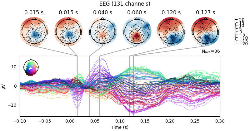
time_start = np.where(evoked.times==-0.1)[0][0]
time_end = np.where(evoked.times==0.3)[0][0]
ch, peak_locs1 = evoked.get_peak(ch_type='eeg', tmin=-0.05, tmax=0.015);
ch, peak_locs2 = evoked.get_peak(ch_type='eeg', tmin=0.015, tmax=0.03);
ch, peak_locs3 = evoked.get_peak(ch_type='eeg', tmin=0.03, tmax=0.04);
ch, peak_locs4 = evoked.get_peak(ch_type='eeg', tmin=0.04, tmax=0.06);
ch, peak_locs5 = evoked.get_peak(ch_type='eeg', tmin=0.08, tmax=0.12);
ch, peak_locs6 = evoked.get_peak(ch_type='eeg', tmin=0.12, tmax=0.2);
ts_args = dict(xlim=[-0.1,0.3]) #Time to plot
times = [peak_locs1, peak_locs2, peak_locs3, peak_locs4, peak_locs5, peak_locs6]
evoked_joint_st = evoked.plot_joint(ts_args=ts_args, times=times);
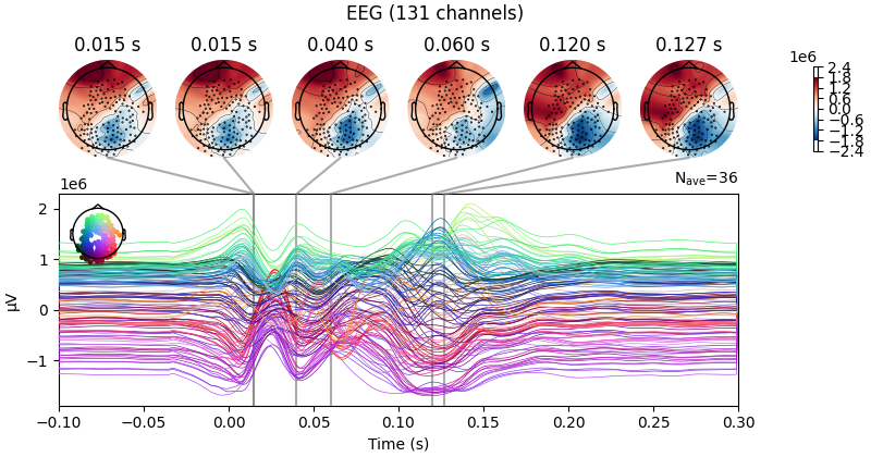
simulated_EEG_st = evoked.copy()
simulated_EEG_st.data[:,time_start:time_end] = F.trainingStats.outputs['eeg_testing']
simulated_joint_st = simulated_EEG_st.plot_joint(ts_args=ts_args, times=times)
Epoch:  0
torch.Size([200, 3, 2])
eeg epoch:  0 loss: 1.5625778 Pseudo FC_cor:  0.5642277474395558 cos_sim:  0.04589348898430153
Epoch:  1
torch.Size([200, 3, 2])
eeg epoch:  1 loss: 0.7566535 Pseudo FC_cor:  0.42674221771625037 cos_sim:  0.26596912245132825
eeg Pseudo FC_cor:  0.8223557710820276 cos_sim:  0.6153893363264156
No projector specified for this dataset. Please consider the method self.add_proj.
No projector specified for this dataset. Please consider the method self.add_proj.
2.3 Virtual_dissection#
url = 'https://github.com/Davi1990/DissNet/raw/main/examples/network_colour.xlsx'
colour = pd.read_excel(url, header=None)[4]
template_eeg = mne.read_epochs(data_folder + '/virtual_dissection/eeg_template.fif', verbose=False)

model_results =np.load(data_folder + '/virtual_dissection/model_results.npy', allow_pickle=True).item()

with open(data_folder + '/empirical_data/dist_Schaefer_1000parcels_7net.pkl', 'rb') as handle:
    stim_region = pickle.load(handle)
stim_region = stim_region['stim_region']

networks = ['Vis', 'SomMot', 'DorsAttn', 'SalVentAttn', 'Limbic', 'Cont', 'Default']
# Create a dictionary to store the network indices
stim_network_indices = {network: [] for network in networks}
for i, label in enumerate(stim_region):
    # Iterate over each network
    for network in networks:
        if network in label:
            stim_network_indices[network].append(i)
            break

# Calculate the number of subplots needed
num_plots = len(networks)
num_rows = 3
num_cols = (num_plots + num_rows - 1) // num_rows

# Set the size of the figure
fig_width = 12  # Adjust as needed
fig_height = 10  # Adjust as needed
plt.figure(figsize=(fig_width, fig_height))

# Loop over networks
for i, network in enumerate(networks):
    # Create subplots
    plt.subplot(num_rows, num_cols, i + 1)

    # Plot standard deviation of EEG test data
    plt.plot(template_eeg.times[200:600], np.mean(np.std(model_results['eeg_test'][stim_network_indices[network]], axis=1), axis=0) - .1,
             color=colour[i], linestyle='--', label='eeg_test')

    # Plot standard deviation of EEG test lesion data
    plt.plot(template_eeg.times[200:600], np.mean(np.std(model_results['eeg_test_lesion'][stim_network_indices[network]], axis=1), axis=0) -.1,
             color=colour[i], label='eeg_test_lesion')

    plt.ylim(0, 0.4)

    # Add title, labels, and legend
    plt.title(f'Network: {network}')
    plt.xlabel('Time')
    plt.ylabel('GMFA')


# Adjust layout to prevent overlap
plt.tight_layout()


# Show the plot
plt.show()

windows = 3

AUC_original = np.zeros((3,model_results['eeg_test_lesion'].shape[0]))
AUC_simulation = np.zeros((3,model_results['eeg_test_lesion'].shape[0]))

for ses in range(model_results['eeg_test_lesion'].shape[0]):

    original_ts = np.std(model_results['eeg_test'][ses], axis=0)

    AUC_original[0, ses] = np.trapz(original_ts[100:137] - np.mean(original_ts[:100]), dx=5)
    AUC_original[1, ses] = np.trapz(original_ts[137:178] - np.mean(original_ts[:100]), dx=5)
    AUC_original[2, ses] = np.trapz(original_ts[178:397] - np.mean(original_ts[:100]), dx=5)


    lesion_ts = np.std(model_results['eeg_test_lesion'][ses], axis=0)

    AUC_simulation[0, ses] = np.trapz(lesion_ts[100:137] - np.mean(lesion_ts[:100]), dx=5)
    AUC_simulation[1, ses] = np.trapz(lesion_ts[137:178] - np.mean(lesion_ts[:100]), dx=5)
    AUC_simulation[2, ses] = np.trapz(lesion_ts[178:397] - np.mean(lesion_ts[:100]), dx=5)


AUC_original[0,:] = AUC_original[0,:] / 37
AUC_original[1,:] = AUC_original[1,:] / 45
AUC_original[2,:] = AUC_original[2,:] / 322

AUC_simulation[0,:] = AUC_simulation[0,:] / 37
AUC_simulation[1,:] = AUC_simulation[1,:] / 45
AUC_simulation[2,:] = AUC_simulation[2,:] / 322


net_AUC_orig = {}
net_AUC_lesion = {}

for network in networks:
    net_AUC_orig[network] = AUC_original[:,stim_network_indices[network]]
    net_AUC_lesion[network] = AUC_simulation[:,stim_network_indices[network]]


AUC_averages_original = np.zeros((len(networks), windows))
AUC_averages_lesion = np.zeros((len(networks), windows))

for idx, key in enumerate(net_AUC_orig.keys()):
    AUC_averages_original[idx, :] = np.mean(net_AUC_orig[key], axis=1)
    AUC_averages_lesion[idx, :] = np.mean(net_AUC_lesion[key], axis=1)


AUC_averages_lesion = AUC_averages_lesion #*100000
AUC_averages_original = AUC_averages_original #*100000


# Create the figure and subplots
fig, axs = plt.subplots(1, 3, figsize=(13, 6))  # 1 row, 3 columns

# Plotting the data on each subplot
for i in range(3):
    axs[i].bar(range(AUC_averages_original.shape[0]), 5 * (AUC_averages_lesion[:, i] - AUC_averages_original[:, i]), color=colour)
    axs[i].set_xticks(range(AUC_averages_original.shape[0]))
    axs[i].set_xticklabels(networks, rotation=45)
    axs[i].set_xlabel('Networks')
    axs[i].set_ylabel('AUC')
    axs[i].set_title(f'Response {i+1}')
    axs[i].set_ylim(-1.5, 1)  # Adjust the y-axis limits as needed

# Adjust layout
plt.tight_layout()


plt.show()

all_lesioned_gfma = np.zeros((model_results['eeg_test'].shape[0], model_results['eeg_test'].shape[2]))
all_original_gfma = np.zeros((model_results['eeg_test'].shape[0], model_results['eeg_test'].shape[2]))


for ses in range(model_results['I_test_lesion'].shape[0]):
        ts2use = (model_results['eeg_test_lesion'] )[ses,:,:]
        all_lesioned_gfma[ses,:] =  np.std(ts2use, axis=0)
        all_original_gfma[ses,:] =  np.std((model_results['eeg_test'] )[ses,:,:]  , axis=0)


net_lesioned_gfma = {}

for network in networks:
    net_lesioned_gfma[network] = all_lesioned_gfma[stim_network_indices[network]]


averages_lesioned = []

for key, value in net_lesioned_gfma.items():
    average_lesioned = sum(value) / len(value)
    averages_lesioned.append(average_lesioned)

averages_lesioned = np.array(averages_lesioned)

# Download the file from the GitHub URL
url = 'https://github.com/Davi1990/DissNet/raw/main/examples/network_colour.xlsx'
colour = pd.read_excel(url, header=None)[4]


fig = plt.figure(figsize=(20, 6))

# Plot the data
for net in range(len(networks)):
    plt.plot(template_eeg.times[200:600], averages_lesioned[net, :], colour[net], linewidth=5)

    #plt.plot(a.times[200:600], averages_lesioned[net, :]- np.mean(averages_lesioned[net, :100]), colour[net], linewidth=5)
    plt.ylim([0.08,0.45])
# Display the plot

plt.show()


2.4 Apply virtual dissection#
# URL of the CSV file containing centroid coordinates for Schaefer2018 atlas
url = 'https://raw.githubusercontent.com/ThomasYeoLab/CBIG/master/stable_projects/brain_parcellation/Schaefer2018_LocalGlobal/Parcellations/MNI/Centroid_coordinates/Schaefer2018_200Parcels_7Networks_order_FSLMNI152_2mm.Centroid_RAS.csv'

# Read the CSV file into a DataFrame
atlas = pd.read_csv(url)

# Extract the 'ROI Name' column from the DataFrame
label = atlas['ROI Name']

# Create a list to store stripped labels
label_stripped = []

# Strip '7Networks_' from each label and append to the list
for xx in range(len(label)):
    label_stripped.append(label[xx].replace('7Networks_', ''))

# Define the list of network names
networks = ['Vis', 'SomMot', 'DorsAttn', 'SalVentAttn', 'Limbic', 'Cont', 'Default']

# Create a dictionary to store the network indices
network_indices = {network: [] for network in networks}

# Iterate over each stripped label
for i, label in enumerate(label_stripped):
    # Iterate over each network
    for network in networks:
        if network in label:
            # Append the index to the corresponding network's list in the dictionary
            network_indices[network].append(i)
            break

# Define the stimulated network
sti_net = 'Default'

# Convert the list of indices for the stimulated network to a numpy array
network_indices_arr = np.array(network_indices[sti_net])

# Get the indices that do not belong to the stimulated network
diff = np.array(list(set(np.arange(200)) - set(network_indices_arr)))

#already trained file
fit_file = data_folder + '/example_fittingresults/example-fittingresults.pkl'


# Define model parameters
state_lb=-0.2
state_ub=0.2
delays_max = 500
when_damage = 80
node_size = 200
batch_size = 20
step_size = 0.0001
pop_size=3
num_epochs = 150
tr = 0.001
state_size = 2
base_batch_num = 20
time_dim = 400
state_size = 2
base_batch_num = 100
hidden_size = int(tr/step_size)
TPperWindow=batch_size
node_size = 200
state_size = 2
transient_num = 10
pop_size = 3

transient_num = 10
final_ouput_P = []
final_ouput_E = []
final_ouput_I = []
final_ouput_eeg = []

# Initialize an empty dictionary to store lesion data
"""lesion_data = {}

# Load data from a pickle file
with open(fit_file, 'rb') as f:
    data = pickle.load(f)

# Initialize the state tensor x0 with random values uniformly distributed between state_lb and state_ub
x0 = torch.tensor(np.random.uniform(state_lb, state_ub,
              (data.model.node_size, pop_size, data.model.state_size)), dtype=torch.float32)

# Initialize the hemodynamic state tensor he0 with random values uniformly distributed between state_lb and state_ub
he0 = torch.tensor(np.random.uniform(state_lb, state_ub,
               (data.model.node_size, delays_max)), dtype=torch.float32)

# Create an input tensor u with zeros, with dimensions 200x10x80xpop_size
u = np.zeros((200, 10, when_damage, pop_size))

# Apply a stimulus of 2000 units to a specific time range (65-75ms) for the first population
u[:, :, 65:75, 0] = 2000

# Create a mask with ones of shape 200x200
mask = np.ones((200, 200))

# Assign the mask to the model's mask attribute
data.model.mask = mask

# Initialize data_mean with ones, with dimensions 1x8x(output_size)x(TRs_per_window)
data_mean = np.ones(([1, int(when_damage / TPperWindow), data.model.output_size, data.model.TRs_per_window]))

# Evaluate the model with the given input tensor u, empirical data data_mean, and initial states x0 and he0
data.evaluate(u=u, empRec=data_mean, TPperWindow=data.model.TRs_per_window, X=x0, hE=he0, base_window_num=100)

# Append the training states for P, E, I, and EEG to their respective final output lists
final_ouput_P.append(data.trainingStats.states['testing'][:, 0, 0])
final_ouput_E.append(data.trainingStats.states['testing'][:, 1, 0])
final_ouput_I.append(data.trainingStats.states['testing'][:, 2, 0])
final_ouput_eeg.append(data.trainingStats.outputs['eeg_testing'])

# Update x0 with the last state of the trainingStats testing states
x0 = torch.tensor(np.array(data.trainingStats.states['testing'][:, :, :, -1]))

# Update he0 by concatenating the reversed first state of the testing states and the remaining part of the original he0
he0 = torch.tensor(np.concatenate(
    [data.trainingStats.states['testing'][:, 0, 0][:, ::-1],
     he0.detach().numpy()[:, :500 - data.trainingStats.states['testing'][:, 0, 0].shape[1]]], axis=1))

# Load data from a pickle file
with open(fit_file, 'rb') as f:
    data = pickle.load(f)

# Create a mask with ones of shape 200x200
mask = np.ones((200, 200))

# Set the mask elements corresponding to network_indices_arr and diff to 0
mask[np.ix_(network_indices_arr, diff)] = 0

# Create an input tensor u with zeros, with dimensions 200x10x(320)xpop_size
u = np.zeros((200, 10, int(400 - when_damage), pop_size))

# Initialize data_mean with ones, with dimensions 1x16x(output_size)x(TRs_per_window)
data_mean = np.ones(([1, int((400 - when_damage) / TPperWindow), data.model.output_size, data.model.TRs_per_window]))

# Evaluate the model with the given input tensor u, empirical data data_mean, initial states x0, he0, and mask
data.evaluate(u=u, empRec=data_mean, X=x0, hE=he0, TPperWindow=data.model.TRs_per_window, base_window_num=0, mask=mask)

# Append the training states for P, E, I, and EEG to their respective final output lists
final_ouput_P.append(data.trainingStats.states['testing'][:, 0, 0])
final_ouput_E.append(data.trainingStats.states['testing'][:, 1, 0])
final_ouput_I.append(data.trainingStats.states['testing'][:, 2, 0])
final_ouput_eeg.append(data.trainingStats.outputs['eeg_testing'])

# Concatenate the first and second elements of the final output lists along axis 1
new_P = np.concatenate((final_ouput_P[0], final_ouput_P[1]), axis=1)
new_E = np.concatenate((final_ouput_E[0], final_ouput_E[1]), axis=1)
new_I = np.concatenate((final_ouput_I[0], final_ouput_I[1]), axis=1)
new_eeg = np.concatenate((final_ouput_eeg[0], final_ouput_eeg[1]), axis=1)

# Read the epoched data from a .fif file
epoched = mne.read_epochs(data_folder + '/empirical-data/example_epoched.fif', verbose=False)

# Compute the average evoked response from the epoched data
evoked = epoched.average()

# Find the index corresponding to the time -0.1 seconds
time_start = np.where(evoked.times == -0.1)[0][0]

# Find the index corresponding to the time 0.3 seconds
time_end = np.where(evoked.times == 0.3)[0][0]

# Load data from a pickle file
with open(fit_file, 'rb') as f:
    data = pickle.load(f)

# Create a copy of the evoked data for simulation
simulation = evoked.copy()

# Replace the simulation data in the time range from time_start to time_end with the EEG testing data
simulation.data[:, time_start:time_end] = data.trainingStats.outputs['eeg_testing']

# Find peak locations in specified time windows and store them
ch, peak_locs1 = simulation.get_peak(ch_type='eeg', tmin=-0.05, tmax=0.015)
ch, peak_locs2 = simulation.get_peak(ch_type='eeg', tmin=0.015, tmax=0.03)
ch, peak_locs3 = simulation.get_peak(ch_type='eeg', tmin=0.03, tmax=0.04)
ch, peak_locs4 = simulation.get_peak(ch_type='eeg', tmin=0.04, tmax=0.06)
ch, peak_locs5 = simulation.get_peak(ch_type='eeg', tmin=0.08, tmax=0.12)
ch, peak_locs6 = simulation.get_peak(ch_type='eeg', tmin=0.12, tmax=0.2)

# Set the y-axis limits for plotting
ymin = -1.8e6
ymax = 1.8e6

# Define plotting arguments with x and y limits
ts_args = dict(xlim=[-0.1, 0.3], ylim=dict(eeg=[ymin, ymax]))

# List of peak locations to highlight in the plot
times = [peak_locs1, peak_locs2, peak_locs3, peak_locs4, peak_locs5, peak_locs6]

# Plot the simulation data with specified arguments and peak times
simulation_st = simulation.plot_joint(ts_args=ts_args, times=times)

# Create a copy of the evoked data for lesion simulation
lesion = evoked.copy()

# Replace the lesion data in the time range from time_start to time_end with the new EEG data
lesion.data[:, time_start:time_end] = new_eeg

# Plot the lesion data with specified arguments and peak times
lesion_st = lesion.plot_joint(ts_args=ts_args, times=times)

# Plot the standard deviation of the EEG testing data across the time dimension
plt.plot(np.std(data.trainingStats.outputs['eeg_testing'], axis=0), label='Intact Structural Connectome')

# Plot the standard deviation of the new EEG data (after virtual dissection) across the time dimension
plt.plot(np.std(new_eeg, axis=0), label='Virtual Dissection', linestyle='--')

# Add labels and title
plt.xlabel('Time Points')
plt.ylabel('Global Mean Field Power')
plt.title('Comparison of GMFP: Intact vs. Virtual Dissection')
plt.legend()

# Show the plot
plt.show()"""
Total running time of the script: (2 minutes 18.114 seconds)