Modelling TMS-EEG evoked responses

This example shows how to organize the empirical eeg data, set-up JR model with user-defined learnable model parameters and train model. After train how to test model with new inputs (noises) to generate simulated EEG. Furethermore, show some analysis based on uncovered neural states from the model.

First we must import the necessary packages required for the example:

# System-based packages
import os
import sys
sys.path.append('..')


# Whobpyt modules taken from the whobpyt package
import whobpyt
from whobpyt.datatypes import Parameter as par, Timeseries
from whobpyt.models.jansen_rit import JansenRitModel,JansenRitParams
from whobpyt.run import ModelFitting
from whobpyt.optimization.custom_cost_JR import CostsJR
from whobpyt.datasets.fetchers import fetch_egtmseeg

# Python Packages used for processing and displaying given analytical data (supported for .mat and Google Drive files)
import numpy as np
import pandas as pd
import scipy.io
import gdown
import pickle
import warnings
warnings.filterwarnings('ignore')
import matplotlib.pyplot as plt # Plotting library (For Visualization)

import mne # Neuroimaging package

Download and load example data

data_dir = fetch_egtmseeg()

Load EEG data

eeg_file_name = os.path.join(data_dir, 'Subject_1_low_voltage.fif')
epoched = mne.read_epochs(eeg_file_name, verbose=False);
evoked = epoched.average()

Load Atlas

atlas_file_name = os.path.join(data_dir, 'Schaefer2018_200Parcels_7Networks_order_FSLMNI152_2mm.Centroid_RAS.txt')
atlas = pd.read_csv(atlas_file_name)
labels = atlas['ROI Name']
coords = np.array([atlas['R'], atlas['A'], atlas['S']]).T
conduction_velocity = 5 #in ms

Compute the distance matrix which is used to calculate delay between regions

dist = np.zeros((coords.shape[0], coords.shape[0]))

for roi1 in range(coords.shape[0]):
  for roi2 in range(coords.shape[0]):
    dist[roi1, roi2] = np.sqrt(np.sum((coords[roi1,:] - coords[roi2,:])**2, axis=0))
    dist[roi1, roi2] = np.sqrt(np.sum((coords[roi1,:] - coords[roi2,:])**2, axis=0))

Load the stim weights matrix which encode where to inject the external input

stim_weights = np.load(os.path.join(data_dir, 'stim_weights.npy'))
stim_weights_thr = stim_weights.copy()
labels[np.where(stim_weights_thr>0)[0]]

Load the structural connectivity matrix

sc_file =  os.path.join(data_dir, 'Schaefer2018_200Parcels_7Networks_count.csv')
sc_df = pd.read_csv(sc_file, header=None, sep=' ')
sc = sc_df.values
sc = np.log1p(sc) / np.linalg.norm(np.log1p(sc))

Load the leadfield matrix

lm = os.path.join(data_dir, 'Subject_1_low_voltage_lf.npy')
ki0 =stim_weights_thr[:,np.newaxis]
delays = dist/conduction_velocity

define options for JR model: batch size integration step and sampling rate of the empirical eeg the number of regions in the parcellation and the number of channels

eeg_data = evoked.data.copy()
time_start = np.where(evoked.times==-0.1)[0][0]
time_end = np.where(evoked.times==0.3)[0][0]
eeg_data = eeg_data[:,time_start:time_end]/np.abs(eeg_data).max()*4
node_size = sc.shape[0]
output_size = eeg_data.shape[0]
batch_size = 20
step_size = 0.0001
num_epochs = 2 # num_epochs = 20
tr = 0.001
state_size = 6
base_batch_num = 20
time_dim = 400
state_size = 6
base_batch_num = 20
hidden_size = int(tr/step_size)

prepare empirical data structure of the model

data_mean = Timeseries(eeg_data, num_epochs, batch_size)

get model parameters structure and define the fitted parameters by setting non-zero variance for the model

lm = np.zeros((output_size,200))
lm_v = np.zeros((output_size,200))
params = JansenRitParams(A = par(3.25),
                         a= par(100,100, 2, True),
                         B = par(22),
                         b = par(50, 50, 1, True),
                         g=par(500,500,2, True),
                         g_f=par(10,10,1, True),
                         g_b=par(10,10,1, True),
                         c1 = par(135, 135, 1, True),
                         c2 = par(135*0.8, 135*0.8, 1, True),
                         c3 = par(135*0.25, 135*0.25, 1, True),
                         c4 = par(135*0.25, 135*0.25, 1, True),
                         std_in= par(np.log(10), np.log(10), .1, True, True),
                         vmax= par(5),
                         v0=par(6),
                         r=par(0.56),
                         y0=par(-2, -2, 1/4, True),
                         mu = par(np.log(1.5),
                                  np.log(1.5), .1, True, True, lb=0.1),
                         k =par(5., 5., 0.2, True, lb=1),
                         k0=par(0),
                         cy0 = par(50, 50, 1, True),
                         ki=par(ki0),
                         lm=par(lm, lm, 1 * np.ones((output_size, node_size))+lm_v, True)
                         )

call model want to fit

model = JansenRitModel(params,
                       node_size=node_size,
                       TRs_per_window=batch_size,
                       step_size=step_size,
                       output_size=output_size,
                       tr=tr,
                       sc=sc,
                       lm=lm,
                       dist=dist,
                       use_fit_gains=True,
                       use_fit_lfm = False)



# create objective function
ObjFun = CostsJR(model)

call model fit

F = ModelFitting(model, ObjFun)

model training given time-varing the stimulus

u = np.zeros((node_size,hidden_size,time_dim))
u[:,:,80:120]= 1000
F.train(u=u, empRecs = [data_mean], num_epochs = num_epochs, TPperWindow = batch_size)

Epoch:  0
epoch:  0 loss: 2.8134632 Pseudo FC_cor:  0.019814780609683346 cos_sim:  0.046948353675922684
Epoch:  1
epoch:  1 loss: 4.681652 Pseudo FC_cor:  0.0018376158472853917 cos_sim:  0.043876568551811594

quick test run with 2 epochs

F.evaluate(u = u, empRec = data_mean, TPperWindow = batch_size, base_window_num = 20)

FC_cor:  -0.010148485106792865 cos_sim:  0.035885374942219904

load in a previously completed model fitting results object run evaluate to generate the simulated eeg with new inputs based on the forward model

full_run_fname = os.path.join(data_dir, 'Subject_1_low_voltage_fittingresults_stim_exp.pkl')
F = pickle.load(open(full_run_fname, 'rb'))
F.evaluate(u = u, empRec = data_mean, TPperWindow = batch_size, base_window_num = 20)

FC_cor:  0.5013935072317343 cos_sim:  0.4067102758116745

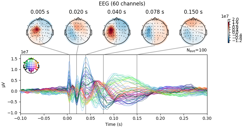
Plot the original and simulated EEG data

epoched = mne.read_epochs(eeg_file_name, verbose=False);
evoked = epoched.average()
ts_args = dict(xlim=[-0.1,0.3])
ch, peak_locs1 = evoked.get_peak(ch_type='eeg', tmin=-0.05, tmax=0.01)
ch, peak_locs2 = evoked.get_peak(ch_type='eeg', tmin=0.01, tmax=0.02)
ch, peak_locs3 = evoked.get_peak(ch_type='eeg', tmin=0.03, tmax=0.05)
ch, peak_locs4 = evoked.get_peak(ch_type='eeg', tmin=0.07, tmax=0.15)
ch, peak_locs5 = evoked.get_peak(ch_type='eeg', tmin=0.15, tmax=0.20)
times = [peak_locs1, peak_locs2, peak_locs3, peak_locs4, peak_locs5]
plot = evoked.plot_joint(ts_args=ts_args, times=times);


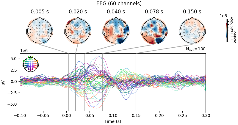
simulated_EEG_st = evoked.copy()
simulated_EEG_st.data[:,time_start:time_end] = F.lastRec['eeg'].npTS()
times = [peak_locs1, peak_locs2, peak_locs3, peak_locs4, peak_locs5]
simulated_joint_st = simulated_EEG_st.plot_joint(ts_args=ts_args, times=times)

• 
• 

Projections have already been applied. Setting proj attribute to True.
Projections have already been applied. Setting proj attribute to True.

Plots of loss over Training (loss should be decressing with nosie)

plt.plot(np.arange(1,len(F.trainingStats.loss)+1), F.trainingStats.loss)
plt.title("Total Loss over Training Epochs")

Plots of parameter values over Training (check if converges)

plt.plot(F.trainingStats.fit_params['a'], label = "a")
plt.plot(F.trainingStats.fit_params['b'], label = "b")
plt.plot(F.trainingStats.fit_params['c1'], label = "c1")
plt.plot(F.trainingStats.fit_params['c2'], label = "c2")
plt.plot(F.trainingStats.fit_params['c3'], label = "c3")
plt.plot(F.trainingStats.fit_params['c4'], label = "c4")
plt.legend()
plt.title("Select Variables Changing Over Training Epochs")

Results Description

The plot above shows the original EEG data and the simulated EEG data using the fitted Jansen-Rit model. The simulated data closely resembles the original EEG data, indicating that the model fitting was successful. Peak locations extracted from different time intervals are marked on the plots, demonstrating the model’s ability to capture key features of the EEG signal.

References

Momi, D., Wang, Z., Griffiths, J.D. (2023). “TMS-evoked responses are driven by recurrent large-scale network dynamics.” eLife, 10.7554/eLife.83232. https://doi.org/10.7554/eLife.83232